AIn this experiment, we will work on relating how light is absorbed by a solution with the concentration of a solute that absorbs light, and how this can be used to determine the concentration of a solute.
Expected Learning Outcomes
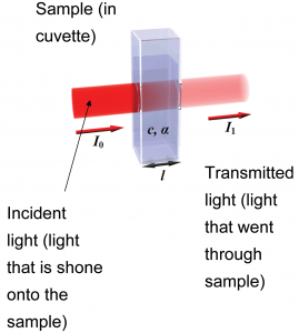
When light is incident on a sample, depending on the electronic structure of the molecule, [1] depending on the wavelength of the incident light some proportion of the light will be absorbed while the rest of the light is transmitted.
To quantify this, we note that – at a particular wavelength – given that the intensity of incident light is , the intensity of light that goes through the sample is ; the rest of this light is absorbed by the sample. The absorbance of the light is related to the intensity of light transmitted by
(1)
Note that is a dimensionless quantity. The absorbance of a substance is typically measured using a spectrometer (of which there are many models). One can plot the absorbance of a solution or substance as a function of the wavelength (i.e. color), as shown in the example below.
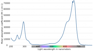
As you will see later when we discuss the electromagnetic spectrum, [2] there is a whole range of different colors which vary in the wavelength of the waves. When light is absorbed, that color of light is therefore removed from what is transmitted.
| Color | Wavelength (nm) |
| violet | 380-430 |
| blue | 430-500 |
| cyan | 500-520 |
| green | 520-565 |
| yellow | 565-580 |
| orange | 580-625 |
| red | 625-740 |
We will explore in this experiment how the color of a substance relates to the wavelength of light absorbed.
As you may have seen before, as the concentration of a solute increases, the color is darker and the amount of light absorbed would have increased. More quantitatively, it can be shown that for a solution with a concentration (molarity, or any other unit) of , the absorbance is related to this by
(2)
where is the path length (the thickness of the solution through which the light travels; this is typically reported in centimeters) and is the molar absorptivity [3] (with units of ). The molar absorptivity varies with wavelength, and is a property of a particular substance at a given wavelength.
The molar absorptivity at a given wavelength can be found by producing a Beer’s Law plot. To do this, solutions of different concentrations of the compound being studied are prepared and their absorbances at the chosen wavelength are plotted (along the -axis) against the concentrations of these solutions (along the -axis).
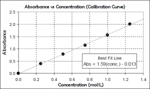
Based on this, the molar absorptivity can be found as the slope of the Beer’s Law plot is equal to . The molar absorptivity of the compound at a given wavelength can therefore be solved as the slope if you know what the pathlength is; most of the time, we use cuvettes with a path length of 1 cm.
Given the molar absorptivity, we can determine the concentration of an unknown solution of the same compound [4] by measuring the absorbance of the sample at the same wavelength as was done for the standard solutions. Given this, we can solve Beer’s Law to find the concentration of the substance.
You should, however, be aware that Beer’s Law only works for relatively low concentrations. Beyond an absorbance of about , the equation breaks down and can no longer be applied. For this reason, concentrations in the experiment should be chosen to have absorbances that are high enough to have a reasonable absorbance, but below the threshold of .
This technique is very widely used in experimental chemistry and is one of the primary ways, for example, by which proteins and nucleic acids are quantified in the biochemical laboratory.
In the first part of the experiment, you will use the PhET Beer’s Law simulation to study how the absorption and transmission of light relate to the color of the substance, as well as obtain a qualitative understanding of how the absorbance relates to the concentration. Select the Beer’s Law option on the simulation.
Each student will be assigned a specific compound to study by your instructor. As part of this experiment, you will share your data with your lab group on the discussion forum. Next week, you will answer additional analysis questions (as a 5-point assignment) that requires you to compare and contrast different spectra.
You are required to prepare two plots using Excel or another spreadsheet program:
The following video outlines how you would make such a plot.
Save the Excel file as this will need to be uploaded to Canvas.
For the same compound, there is a preset wavelength where the optimal wavelength is found; select this mode and record the wavelength.
Measure the absorbance at a number (at least 5) of concentrations and record your measurements. What happens qualitatively to the amount of light that shines through the cuvette?
You are urged to select a range of absorbances such that the maximum absorbance is approximately 1.This is explained in the following video:
Like in the last exercise, you are required to share the Beer’s Law plot with your lab group.
While in the last part you were able to visualize the trends better and to investigate different solutions, it has two different flaws:
To do this, you will use the spectrophotometry virtual lab by Gary L. Bertrand. In this virtual experiment, you will prepare a Beer’s Law plot for one of the two solutes and then study the absorption spectrum. This simulates the operation and use of an old Spectronic 20D spectrophotometer.
On the right, you will see a rack with five test tubes.
In the actual laboratory, the vast majority of spectrophotometers today use square cuvettes that can be made of plastic, glass or quartz and are square in shape. When you do the experiment in real life, you should (a) take care not to break glass/quartz cuvettes (these are very expensive and fragile), (b) make sure that the clear sides of the cuvettes are aligned with the light beam (usually there are two glazed sides), and (c) hold the cuvette on the glazed sides carefully with your fingers so fingerprints do not block the optical path.
The Spectronic 20D is set such that the light path is blocked when there is no test tube in the light path. This is a convenient way of calibrating the spectrometer so that 0% transmittance is a set level of light, accounting for the presence of stray light due to imperfections in the detector. Similarly – and this is true of all spectrophotometers – you need to zero the spectrometer so that the absorbance of a solution with zero solute is read as zero.
Please watch this video by Mark Garcia which demonstrates the use of the Spectronic 20D:
Here is a diagram of the controls on this spectrophotometer:
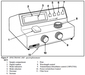
The zero control and the transmittance/absorbance control knobs at the front will not give you exactly 0% transmittance/0 absorbance. You are asked to set these to as close as possible.
In this part of the experiment, you will determine the wavelength where the absorption maximum occurs.
You are given two stock solutions: a 13.0 ppm stock solution of the red dye and a 10.0 ppm stock solution of the blue dye. You are also given some solvent.
You will need to use the appropriate standard solution for your unknown.In this part of the experiment, you will obtain data needed to create a Beer’s Law curve.
To prepare solutions of different concentrations, you need to:
Click on the “dump solutions” link at the right hand side if you have no more empty tubes left. This will give you more empty tubes to work with.
To obtain the concentration in a given test tube, you can solve for this using the equation you’ve seen in class for dilution calculations
(3)
Here, instead of having concentrations in molarity, you will have concentrations in ppm. This will affect the units on the -axis of your Beer’s Law plot, but not the actual calculations.
The path length will be 1 cm. You can use the same procedure as above to find the slope of the Beer’s Law plot.
Put tube 4 into the spectrophotometer and record the concentration. You can then use the absorbance found and the slope of the plot from the previous part to find the concentration of the dye in ppm for your unknown.
Virtual Chemistry Experiments Copyright © by Yu Kay Law. All Rights Reserved.